Carnival Of Mathematics

In this somewhat different post, I am hosting the long-running Carnival of Mathematics. First I’ll talk about 223 (the issue number) and then I’ll round up some mathematical posts from December 2023.

It’s primetime we talk about 223. First of all, it is a lucky prime, to which it is unknown if there are infinitely many. To write the number 223 as the sum of fifth powers requires 37 terms, more than any other number. This is an example of Waring’s problem has a rich history going back to Diophantus nearly 2000 years ago. Also, 223 is the number of permutations on 6 elements that have a strong fixed point (see below for Python code).

And now for what happened last month.

• Quanta brings current research mathematics to a general audience. Solutions to long-standing problems happen all the time in math, and this video highlights some from the past year. The one I know the most about is at the end. The “Dense Sets have 3-term Arithmetic Progressions” problem has been the subject of intense study for over 70 years. Multiple Fields medal winners over several generations have studied the problem and a big breakthrough was made by two computer scientists (including a PhD student from my Alma mater).
• Quanta also posted their Year in Math. Particularly interesting to me is Andrew Granville’s (my former Mentor) discussion of the intersection of computation and mathematics.
• Here you can find a “Theorem of the Day,” where the author impressively keeps posting interesting theorems from mathematics on a daily basis.
• An interesting story of a Math SAT problem with no correct answer.
• John Cook’s explanation of a Calculus trick. See if you can figure out how his trick is a manifestation of the fact that for a right triangle with angle , only depends on the ration of the non-hypotenuse sides.
• If you are interested in some drawings with math and a little bit of humor, you can find that here.
• Another article from Quanta highlighting a very recent breakthrough. Interesting to me is how quickly (3 weeks!) the result was formalized into computers. What this means is a group of people got together and input all of the results into a computer which then tested the validity of the results in an automated way. This process of inputting the results into the computer can be quite painful and I am impressed by the speed at which it was done. You can check out my previous blog post for my experience with it. Incidentally, one of the classical results I helped formalized in that blog post was used to formalize the recent result. The referee and review process for math papers is particularly painful for mathematicians. It is not uncommon to see mathematicians submit a paper and wait years for the decision to accept or reject to come in. Meanwhile, especially for younger mathematicians, their career hangs in the balance as they await these decisions. Adopting Software Engineering best practices to this process, as done above, I believe go a long way to alleviate some of this anguish.

Here is the Python code for the strong fixed point verification.

from itertools import permutations
perms = permutations([1,2,3,4,5,6])

def fixed_points(perm):
    """
    Input: a permutation written as a tuple, i.e. (1,3,2) for 1->1, 2->3, 3->2
    Output: a list of the indices of the fixed point of the permutation
    """
    return [ind for ind,p_ind in enumerate(perm) if ind+1 == p_ind]

def is_strong_fixed_point(ind,perm):
    """ 
    Input: An index and a permutation 
    Output: True if the index is a strong fixed point of the permutation, else False
    See here: https://oeis.org/A006932
    """
    for lesser_ind in range(0,ind):
        if perm[lesser_ind] > perm[ind]:
            return False
    for greater_ind in range(ind+1,len(perm)):
        if perm[greater_ind] < perm[ind]:
            return False
    return True

counter = 0 
for perm in perms:
    for fixed_point in fixed_points(perm):
        if is_strong_fixed_point(fixed_point,perm):
            counter +=1 
            break 
print(counter)

Temperature in Natural Language Processing

In Machine Learning, and in particular Generative AI, temperature is a useful hyperparameter for tuning model outputs.

In this post, we will discuss the following.

• Temperature is a parameter developers can use to alter outputs from Large Language Models
• With a higher temperature we get more creative outputs.
• Why changing the temperature is useful.

Let’s start with an example (the code I used is at the end of this post). Consider the following prompt, taken from Google’s Minerva paper.

A line parallel to passes through . What is the -coordinate of the point where this line crosses the -axis?

I asked ChatGPT four times to answer this prompt, similar to what was done in their paper. Here is what I got:

• Since a line parallel to has the same slope, the desired line has slope 4. Therefore, the equation of the line is of the form . Plugging in the point , we have , so . Therefore, the -intercept is .
• Since the line is parallel to , which has a slope of 4, the line must have a slope of 4. The equation of the line is then . Setting , we find .
• The given line has slope 4, so a line parallel to it also has slope 4. If a line with slope 4 passes through , then it is of the form . Expanding the right side gives , so . Setting , we find that the line crosses the -axis at .
• Since a line parallel to will have the same slope, this line will have slope equal to 4. Therefore, its -intercept has -coordinate .

The first three answers are correct, while the last answer is wrong. Actually the final answer is correct all the way up to the 4 in 14. What happened under the hood is that likely ChatGPT was nearly sure the 4 should be a 0, but still was hedging its bets that it could in fact be a 4. In that particular instance, it randomly chose the 4.

To understand temperature, we first have to understand a bit about how large language models work. For instance, the G in GPT stands for generative. In practice, this means that given some text, the Large Language model will try to predict the next letter (or more precisely token, see this previous blog post). For a model like GPT, each letter will be assigned a probability as to how likely it is to be the next character. For instance, in the example above, the model likely assigned a large probability to the character 0 and a small, but positive, one to the character 4. It’s at this point the concept of temperature is useful.

Now that we have a bunch of probabilities assigned to each character, we have to define a methodical way of choosing the next character. Do we just assign the character with highest probability?

Unfortunately, there is no “one size fits all” solution to this problem, which is why we introduce the notion of temperature. Let’s look at an example. Suppose we are choosing between two characters to output next. Suppose further that our model overwhelming thinks the first character is the best choice. We plot how the temperature affects our choice of character in this example.

Here, for a low temperature (i.e. close to 0), the model outputs the first character nearly all the time. But as the temperature grows larger, the model outputs each character around half the time.

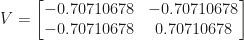
Thus as we decrease the temperature, we get closer to the model that only outputs the highest probability character. As we increase the temperature, we get closer to the model that chooses each character randomly and uniformly.

And just for completeness, I will mention that the temperature 0 response I got from ChatGPT in the above example was in alignment with the three correct answers.

Why is Temperature Useful?

The argument made in the aforementioned Minerva paper was that by increasing the temperature, we can have the model generate a variety of outputs. From this variety of outputs, we may pick the “best” one. How we choose the best one can vary, but what they did is just take the most popular one.

This allows us to explore the probability space of answer generated by the generative model in order to make a more informed decision at which one to proceed with.

The Code

Here is the Python code I used to generate the example above. First I created a .env file in the same directory with my Open AI API key (fill out with your API key)

OPENAI_API_KEY=

Then I used Langchain (though this is not really required for such a simple example) as follows:

import os 
from langchain.chat_models import ChatOpenAI
from langchain.chains import LLMChain
from langchain import PromptTemplate

OPENAI_API_KEY = os.environ.get("OPEN_API_KEY")

query = "A line parallel to $y = 4x + 6$ passes through $(5, 10)$. What is the $y$-coordinate of the point where this line crosses the $y$-axis?"

prompt = PromptTemplate.from_template(query )
prompt.format()
llm = ChatOpenAI(temperature = 1)

chain = LLMChain(llm=llm, prompt=prompt)

responses = [chain.run({}) for _ in range(5)]

Singular Value Decomposition and PCA

Principal Component Analysis (PCA) is a popular technique in machine learning for dimension reduction. It can be derived from Singular Value Decomposition (SVD) which we will discuss in this post. We will cover the math, an example in python, and finally some intuition.

The Math

SVD asserts that any matrix can be written as

where

• is and is rectangular diagonal, that is for .
• and are orthogonal, that is and .

This allows us to derive PCA. First, we are given a data matrix, , that is a matrix where each of the rows are data points with features.

First, we translate each column of so that each column has mean zero. That is we translate each column by , respectively. For instance if

Then we would translate the first column by -3 and the second column by -4. Then we divide each column by their standard deviations, . Thus in our example we divide the first column and second column by . Let us call this new scaled matrix to align with our notation above. Then we can perform PCA by performing SVD

and computing the $m \times d$ matrix

For PCA with components, the data point in the row of is transformed to the first entries of the row of .

Put another way, given a data point , we compute PCA in two steps:

and then

where are the first columns of .

Python Example

We will show how to code up PCA using only numpy and torchvision (only to retrieve some classical datasets). First we start with some imports.

import torchvision.datasets as datasets
import numpy as np 
import matplotlib.pyplot as plt
import seaborn as sns 

Then we define a PCA function that does the work we did in the previous section. The data is inputted as a numpy array. We utilize the np.linalg.svd function for SVD and specify full_matrices=False so that the dimensions of and align with our computations above.

def pca(data,k=2):
    data = data.reshape((data.shape[0], -1))
    mu = np.mean(data, axis=0)
    std = np.std(data, axis=0).clip(min=1e-10).reshape(1,-1)
    A = (data - mu) / std
    U, S, Vt = np.linalg.svd(A, full_matrices=False)
    V = np.transpose(Vt)
    tmp = np.dot(A, V)
    return tmp[:,:k],V

We can now load in the MNIST, Fashion MNIST, and CIFAR datasets from torchvision datasets.

mnist = datasets.MNIST(root='./data', train=True, download=True, transform=None)
np_mnist = mnist_trainset.data.numpy()/255.0

fmnist_trainset = datasets.FashionMNIST(root='./data', train=True, download=True, transform=None)
fmnist_numpy = fmnist_trainset.data.numpy()/255.0

cifar= datasets.CIFAR100(root='./data', train=True, download=True, transform=None)
cifar_np = cifar.data /255.0

We can now perform PCA on these datasets.

pca_mnist,V_mnist = pca(np_mnist)
pca_fmnist , V_fmnist = pca(np_fmnist)
pca_cifar , V_cifar = pca(cifar_np)

We can see how they divide the datasets into their classes. With the following code.

fig, axs = plt.subplots(3, 4, figsize=(15, 6))

for i in range(3):
    for j in range(4):
        N = i*4+j 
        axs[i, j].imshow(.5*V_mnist[:,N].reshape((28,28))+.5, cmap="gray")
        N +=1 
        if N == 1:
            axs[i, j].set_title(f"{N}st Principal Component")
        elif N == 2:
            axs[i, j].set_title(f"{N}nd Principal Component")
        elif N == 3:
            axs[i, j].set_title(f"{N}rd Principal Component")
        else:
            axs[i, j].set_title(f"{N}th Principal Component")
        axs[i, j].axis('off')

We can also see what pixels are activated for each principal component. For instance we have the following for the MNIST data set

and the Fashion MNIST

You are encouraged to think about how I came about these images!

Intuition

There are two steps to PCA:

• Scaling the columns of the data matrix
• Computing the SVD and transforming the data

Let’s see these steps with a text example to see what’s going on. We generate a bunch of points in 2 dimensional space that lie close to the line , where is between 0 and 1.

import numpy as np 

X = np.zeros((1_000,2))
X[:,0] = np.random.uniform(0,1,1_000)
X[:,1] = 2*X[:,0] + np.random.normal(0,0.1,1_000)
fig = sns.scatterplot(x = X[:,0],y = X[:,1])

Now we perform the scaling step.

Z = (X - np.mean(X, axis=0)) / np.std(X, axis=0)
fig = sns.scatterplot(x=Z[:, 0], y=Z[:, 1])

You can see first of all this shifted the data so that now the center point is , instead of the original . Also, through scaling, the data now lies near the line , rather than .

The scaling step (in particular division by the standard deviation) makes it so we do not favor a feature simply because the coordinates are on average larger.

We can now compute .

Vt = np.linalg.svd(Z, full_matrices=False)[-1]
V = np.transpose(Vt)

This gives

Notice the first column of , is a scalar multiple times

and the second column, is a scalar multiple of

.

Here is what is going on. In our data set, after scaling, data points lie on the line , up to a small error. PCA is a way of automating the process of finding this line. Indeed, this is given by the vector . When we compute , for a data point , we are getting information on the whereabouts of lies on the line . Indeed, for a point we have

so this dot product is able to precisely compute where is on the line .

In higher dimensions, the same general principle holds. PCA allows us to find the line (or plane, or higher dimensional space) that best describes our data. Indeed let’s look at the previous example in 3-dimensions. We just add some small random noise to the additional coordinate

X = np.zeros((1_000,3))
X[:,0] = np.random.uniform(0,1,1_000)
X[:,1] = 2*X[:,0] + np.random.normal(0,0.1,1_000)
X[:,2] = .1*np.random.uniform(0,1,1_000)
Z = (X - np.mean(X, axis=0)) / np.std(X, axis=0)
Vt = np.linalg.svd(Z, full_matrices=False)[-1]
V = np.transpose(Vt)
print(V)

Here we find that the first column of is, roughly, a scalar multiple times

Thus PCA still identifies the important relation between the first and second coordinate (after scaling) and disregards the other noise.

Limitations of PCA

One major limitation of PCA is that it’s only capable of capturing linear relations between the features. This could be handled by combining feature engineering with PCA, though this presents its own set of challenges. One way to overcome this is to invoke non-linear methods of dimension reduction, i.e. t-SNE or UMAP. In the following figure, I ran t-SNE on the MNIST data set (first using PCA to reduce the number of features to 25). We can see it performs much better than PCA at identifying digits.

Furthermore, PCA can lead to unpredictable outcomes that depend on the distribution of the data collected, as studied in this paper of Elhaik which I learned about from the Batch. This highlights that one should be careful making inferences from PCA alone.

The Square Root Cancellation Heuristic

In the first equation of the popular Attention is all you need paper (see also this blog post), the authors write

In this post we are going to discuss where the comes from, leading us to some classical Probability Theory. We will first talk about the math with some examples and then quickly make the connection.

The principle of square root cancellation also appears in the Batch Norm Paper, Neural Network weight initialization (see also Xavier Uniform), and elsewhere.

The Math

Let be a $d$-dimensional vector with entries that are either or Then we may write

We will be interested in the simple question: what is the sum of the coordinates? For a fixed vector, we can easily compute this via

The largest this sum can be is and the smallest it can be is . However, what we would like to know the average behavior of this sum

Since the vector has both ‘s and ‘s, there will likely be cancellation in the sum. That is, we expect the sum will not be either or . It turns out that as gets large, there will typically be a lot of cancellation.

Let’s first run an experiment in python. We let and compute the sum of 100,000 random vectors each with entries.

import numpy as np 
import seaborn as sns 

d = 500; sums = []

for _ in range(100_000):
    v = np.random.choice([-1, 1], size=d)
    sums.append(np.sum(v))

_ = sns.histplot(data = sums)

We see that most of the sums are quite a bit smaller than 500, and barely any are smaller than or larger than 75.

This is the so-called square root cancellation. If we take a random vector of dimension with randomly generated entries, we expect the order of the sum to be . Here , and it is a general phenomenon that most of the sums will lie between, say, and . This general principle goes much deeper than vectors and turns out to be very well-studied concept in several areas of mathematics (see this post for Number Theory or this post for Probability). In fact, the famous Riemann Hypothesis can be reformulated as showing a certain sum exhibits square root cancellation.

The square root cancellation heuristic asserts that “most” vectors exhibit square root cancellation. Put another way, if we come across a vector in practice, we’d expect there to be square root cancellation as in the above example.

It turns out that the example we will discuss below generalizes considerably. The only thing that really matters is that each coordinate has mean zero (which is easily remedied by translation of a fixed constant). There are also some technical assumptions that the coordinates of are not too large, but this is never an issue for vectors that only take on finitely many values. The motivated reader can consult the Lindeberg-Lévy Central Limit Theorem for more along this direction.

Before going any deeper, let’s explain what’s going on in the aforementioned Attention is All you Need paper.

Attention is All You Need Example

In the above equation, we have

Each entries of is the dot product a row of and a row of :

It turns out that this is the sum of numbers, and by the square root cancellation principle, we expect the sum to be of order . Hence dividing through by this number allows the sum to be, on average, of size comparable to 1 (rather than the much larger .

Keeping the sums from being too large helps us avoid the problem of exploding gradients in deep learning.

Back to the Math

Recall we had a vector of dimensions,

and we are interesting in what the sum is, on average. To make the question more precise, we assume each coordinate is independently generated randomly with mean zero. The key assumption is independence, that is the generation of one coordinate does not impact the others. The mean zero assumption can be obtained by shifting the values (for instance instead of recording a six sided dice roll, record the dice roll minus 3.5).

Here are some examples in python that you are welcome to check

v1 = np.random.choice([1,2,3,4,5,6],size=500) - 3.5
v2 = np.random.exponential(1,size=500) - 1 
v3 = np.random.normal(0,1,size=500) 

For such a vector, and a bit large (say over 30), we expect

Specializing to the case where the coordinates are , we recover the from earlier. Now why should we expect that the sum is of size ?

One way to see this is to explicitly compute the expected value of

which is precisely $d$. This computation can be done by expanding the square and using that the covariance of two different coordinates is 0. We will put the classical computation at the end of the post for those interested.

It is a common theme in this area that working with the square of the sum is theoretically much easier than working with the sum itself.

The Central Limit Theorem

It is worth reiterating that the square root cancellation heuristic generalizes much further than the example, but let’s continue our focus there. The astute reader will notice that the above histplot looked like the normal distribution. In fact, it is. If we consider the sum

the histplot will be normal with mean zero and variance. Put another way,

and we can quantify the precisely. Thus if we have a sum of numbers (where we expect the numbers to be on average 0), we can divide the sum by in order to make the sum .

The Variance Computation

We will show

Indeed,

using FOIL from algebra and linearity of expectation. It is thus enough to show,

for every . But this follows from independence.

How Does ChatGPT read?

How would ChatGPT read the infamous “Hello, World!” Does it see each character, sequentially

H e l l o , W o r l d !

Or maybe it sees each word as well as the punctuation:

Hello , World !

By the end of this post we will have a full understanding of this. On the way, we will learn about unicode, UTF-8, and byte pair encoding (BPE).

In order to understand how ChatGPT sees data, we have to understand the data on which it is trained on. The majority of the data used to train GPT-3 comes from the Common Crawl dataset, which is text scraped from the internet. Thus we turn our attention to understanding how text is encoded on the web.

Code Points

In order for our computers to store and transfer text, we need a way of converting characters (i.e. elements of an alphabet, punctuation, etc.) to bits. Thanks to binary numbers it is enough to convert characters to integers (though encoding schemes like the popular UTF-8 provide a more complex and efficient conversion code points to bits, as we will see later).

Thus we first turn our attention to mapping characters to integers, denoted a character encoding. This leads us to Unicode.

A Brief History of Unicode

The earliest character encoding was ASCII (pronounced like as-kee), which stands for the American Standard Code of International Information Exchange. One key problem with it is already evident from the name..what if non-Americans would like to exchange information?

ASCII provides code points for 128 characters, including the English alphabet and common punctuation. ASCII is typically sufficient for sending English messages. You can get the ASCII encoding of the letter A (and vice versa) in python with the following built in function.

print(ord("A")) #ASCII code point of A
print(chr(65)) #character of code point 65

In addition to the aforementioned symbols, there are also code points that correspond to non-printable information, which can cause some confusion.

ASCII contains most of the characters you will need if your goal is to communicate in English, and was widely adopted in the 1960s. However, ASCII cannot support languages with a different alphabets, accented characters, emojis, and more.

Thus a group of people set to create more inclusive standards for representing text, that was also backwards compatible with the already widely adopted ASCII. After several iterations, Unicode is now the widely adopted standard. It is supported by a variety of blue chip companies, as can be seen from their member’s page.

What is Unicode?

Unicode is a way to convert nearly 150,000 characters to integers. For instance, here is a nice list of the integer to character conversions. You can input unicode directly into html via &# followed by the decimal representation. For instance.

<p>&#70000</p>
<p> &#70000 </p>

renders as 𑅰 and 🤠, respectively.

You can also directly write unicode on your local machine by following a tutorial (Mac, Windows, and Linux).

Thus Unicode extends ASCII to accommodate nearly all desired written text with nearly 150,000 characters assigned a code point. It turns out this encoding plays a large part in encoding text in the web and consequently the training of ChatGPT. But before we see this connection, we have to discuss UTF-8.

UTF-8

While unicode is accommodating in terms of encoded characters, it is not terribly efficient. For instance, if you plan to write in mostly ASCII, it would make sense to make those characters require a smaller amount of space to encode. This is exactly the purpose that the UTF-8 encoding serves.

Recall that to store and send text, one needs to convert to bits. In practice, we work with bytes, which is just 8 bits. As 8 bits gives possibilities, all of ASCII can be represented by 1 byte (with room to spare). UTF-8 is an attempt to convert the Unicode code points to bytes in an efficient manner.

A byte can be represented by two hexadecimal numbers. For instance, 0-20 are given by:

0 1 2 3 4 5 6 7 8 9 A B C D E F 10 11 12 13 14

So we can represent the character H, which is 72 in ASCII, by 48 in hexadecimal. UTF-8 converts Unicode code points to either 1,2,3 or 4 bytes. For instance, the UTF-8 encoding of

Hello 🤠

is

48 65 6c 6c 6f 20 f0 9f a4 a0

Note that the first 5 bytes correspond to H e l l o, while the last 4 correspond to 🤠. UTF-8 is set up in such a way that it is clear the last 4 bytes are all part of one character.

Back to Chat GPT

Unicode has the advantage of being able to methodically encode nearly all text on the web to integers. An integer turns out to be perfect for inputting into a machine learning model. However, inputting raw Unicode, which consists of nearly 150,000 characters, would be inefficient and beyond current computational power. For instance, the encoding used for ChatGPT that we will discuss below has 100,261 tokens. Thus it is convenient to have a clever way of converting text to integers that goes beyond Unicode.

Byte Pair Encoding (BPE) is a preprocessing step that allows us to identify subwords that appear often in the text. The starting point of BPE, as the name suggests, is bytes. We start by encoding every single byte to an integer 0-255, which we call a token. Thus any Unicode text can be written as a sequence of tokens via the UTF-8 encoding. For instance, the Hello 🤠 above can be tokenized to

72 101 108 108 111 32 240 159 164 160

However, we can make this more efficient by adding additional tokens. For instance, the word “to” appears quite often in English text. However, it is currently encoded as

83 78

What we can do is create a new token for the word to so that instead of using 2 tokens for this common word, we only use one (this is the “pair” in BPE). Using tiktoken, released by openai, we can see that this is exactly what was done.

#will need to install tikoken: pip install tiktoken 
import tiktoken 
enc = tiktoken.encoding_for_model("gpt-3.5-turbo") #gpt-3.5-turbo - ChatGPT
enc.encode('to')

Running this code, we see that the integer 998 is reserved for to.

Byte Pair Encoding

So how exactly is the byte pair encoding performed? We will give a brief explanation and note the details can be found in ~20 lines of python code in Algorithm 1 of this paper of Senrich, Haddow, and Birch and also explained in Section 2 of the gpt-2 paper.

We start by taking a smallish sample of our text data. We then convert convert the text to bytes via the UTF-8 decoding. After this we see which pair of bytes appears the most often and assign a new token to that pair. We can see the first pair with the following python code (continued from above).

print([x for x in enc.decode_bytes([256])])

The result is 32 32, which corresponds to two consecutive spaces. BPE then repeats this process, with the possibility of joining the newly created token to any other token. In fact, this is repeated over 100,000 times!

We see that the first join is joining bytes 32 with itself. In fact, this is just two consecutive spaces. The first non-space join is that of i and n to form “in” (token 258).

It is worth mentioning that BPE is not the only method of tokenizing. For instance, Google’s Bard uses SentencePiece.

One Issue

It is well known that not every byte sequence is valid UTF-8 code. Thus, it is possible in theory for ChatGPT to produce non-valid UTF-8. Of course, this becomes increasing rare as the model is trained more and more. In fact the decoder provided by tiktoken has a kwarg to specify how to address this exact issue.

Recap

To see how ChatGPT is trained, we first have to understand the data. The data is scraped from the web, which lead us to the UTF-8 encoding. Such an encoding gives nearly 150,000 characters and is inefficient. This motivates looking at a compression technique, i.e. the Byte Pair Encoding.

Using AI to Write Math

Unfortunately (or perhaps, fortunately), we are still far from the days where we can ask a computer to write proofs for us. However, there are tools available today that can concretely assist with writing mathematics.

I made a video on the topic, with blog post below.

While I left research mathematics some time ago, I still find myself typing up some math from time to time. For me this has become a bit easier with Github Copilot.

I am now VSCode as my text editor to write LaTex. VSCode is a free and powerful IDE used by millions of software engineers. With it, one can access GitHub Copilot (for $100/year).

GitHub Copilot saves quite a bit of time in Latexing. Let’s see it in action suggesting useful LaTex code for a matrix.

The lighter text “\begin{pmatrix}” is what is suggested by Github Copilot. You can simply hit tab to accept the suggestion or keep typing to reject it. Let’s keep accepting:

This eventually gives the final result.

As you can see it quite accurately gives the LaTex code for a matrix, and only takes about 3 seconds real-time to do so.

Funny enough, it suggests some non-sense afterwards, about having integer entries and some other things.

Vscode has a lot of flexibility in itself. There are many extensions that are useful. For instance, to work with latex, you’ll at the very least need a latex and pdf viewer extension. There is also git integration, which allows you to store your work remotely with the click of a couple of buttons.

Another reason to get familiar with VSCode is that it is a powerful tool for programming. That way, if you do every need to do some programming, you will already have a leg up on getting started!

Truthfulness of AI models like Chat GPT

Large language models, have improved and become more main stream. I discuss this in the video below with AI Researcher Xavier Garcia.

I started a YouTube Channel

My First Video

I am happy to announce that I just posted my first video to a new YouTube Channel. The result is an interview with Xavier Garcia about how Chat GPT works.

What’s Next?

I’ll continue to post videos surrounding Machine Learning, Data Science, and perhaps elsewhere. I plan to do more interviews, individual videos about relevant topics, as well as some educational material.

The Process

I was already meeting with Xavier regularly to discuss Machine Learning topics, and so I thought to myself that other people might benefit from our discussions.

Our discussion for the video was perhaps a bit altered than the usual, as we were a bit less likely to say things “off the cuff.” I’ll be looking to make this easier going forward, as I think a lot of valuable insight lie here.

There was/is a learning curve in making videos, and I’ll definitely be looking to improve the quality as time goes forward. From zero to published video took a couple months (of course not doing this full time). Also, I got lucky and found a very helpful video editor which made things a lot easier. Things like sound quality, video quality, and lighting are not things I’ve had to worry about too much in the past. I didn’t invest too much in equipment, just trying to make use of what I had.

Can Chat-GPT Do Math?

Chat-GPT is a new impressive AI chatbot released by Open AI. Impressive applications of it can be found all over the internet. But can it do math?

By math, we do not mean simply perform computations. Its own design ensures that there will be computational problems it will be unable to solve. What I am more interested in is if it can solve problems that require some mathematical reasoning.

To choose our problems, we use the MMLU dataset. Galactica, a large language model recently released by Meta AI, has achieved some good results on this dataset. Their findings are in section 5.3 of their paper.

In what follows, we’ll pick a few problems and see how Chat-GPT handles them. If it fails, we will try to reword the question in hopes of achieving some partial results.

We note that the MMLU data set has multiple choice questions, but we just present the questions to chat-GPT. We just choose question from the abstract algebra section of the MMLU. Afterwards, we’ll prod chat-GPT for intuition and a proof. We’ll end by suggesting a few applications of chat-GPT for mathematicians.

Question 1

Me: The inverse of -i in the multiplicative group, is

Chat-GPT: The inverse of -i in the multiplicative group is . The inverse of an element in a group is an element such that $latex xy=yx=1$, where is the identity element of the group. In this group, is the identity element, so the inverse of an element is an element such that .

For example, the inverse of is , because . Similarly, the inverse of is , because .

Remark: Chat-GPT answers this question perfectly and gives an excellent explanation. To be fair, this is an easier question.

Question 2

Me: How many homomorphisms are there of Z into Z_2? Please write in latex format.

Chat-GPT: There are two homomorphisms of into . They are defined as follows:

such that for all

such that for all

Remark: Again, Chat-GPT is spot on. However, I asked this question a few times and it once said 1, and another time said two but gave a false justification:

There are only two homomorphisms of Z (the integers) into Z2 (the integers modulo 2).

One homomorphism sends every integer to 0, and the other homomorphism sends every integer to 1.

Question 3

Me: Let p = (1, 2, 5, 4)(2, 3) in S_5 . Find the index of <p> in S_5. Please write your answer in latex.

Chat-GPT:

The index of <p> in S_5 is the number of elements in S_5 that come before <p> in lexicographic order.

To find the index of <p>, we must first determine the cycle type of p. The cycle type of a permutation is a list of the lengths of its disjoint cycles, listed in decreasing order.

The cycle type of p is [2,2], since p consists of a 2-cycle and a 2-cycle.

Now we can use the cycle index of S_5 to determine the number of permutations in S_5 with cycle type [2,2].

The cycle index of S_5 is given by:

where is the number of permutations in S_5 with i cycles, and is a variable representing a cycle of length i.

Substituting the cycle type [2,2] into the cycle index gives:

This simplifies to:

The coefficient of in this expression is , so the number of permutations in S_5 with cycle type [2,2] is .

Since <p> is the only permutation in S_5 with cycle type [2,2], it is the -th permutation in S_5.

Therefore, the index of <p> in S_5 is .

Remark: Woah! This is very wrong! The very first sentence is completely wrong. Also, its final conclusion, is not even an integer, which is certainly not right. Indeed, the index of a subgroup counts something and most be a positive integer.

We are able to salvage something though. Suppose we computed that the order of is 5, using our algebra skills. Then we can prompt chat-GPT with the following.

Me: Now suppose is a subgroup of order 5. What is the index of in ?

Chat-GPT: The index of a subgroup in a group is the number of left cosets of in . This is also equal to the number of right cosets of in .

Since the order of a subgroup divides the order of the group, the order of must divide the order of , which is 120. The only divisors of 120 that are less than 120 are 1, 2, 3, 4, 5, 6, 8, 10, 12, 15, 20, 24, 30, 40, and 120. Therefore, the only possible orders for are 1, 2, 3, 4, 5, 6, 8, 10, 12, 15, 20, 24, 30, 40, and 120.

Since the order of is 5, the index of in is .

Remark: Here chat-GPT answers perfectly with a great explanation. Perhaps it would be nice to mention that the main fact being used is Lagrange’s theorem, though this can easily be obtained by asking it “What theorem did you use above?”

But what’s the intuition?

What makes a research mathematician great is a certain “intuition” for problems. Let’s see if chat-GPT can explain any of that.

Me: Can you explain the intuition behind the Cauchy-Schwarz inequality? Please write any math formula in latex.

Chat-GPT: Sure! The Cauchy-Schwarz inequality is a useful inequality that arises in various areas of mathematics, such as vector algebra, inner product spaces, and probability theory. It states that for any two vectors x and y, the following inequality holds:

Intuitively, the Cauchy-Schwarz inequality states that the inner product of two vectors x and y is “controlled” by the lengths of the vectors x and y. To see this, consider the special case where x and y are unit vectors (i.e., vectors of length 1). In this case, the inequality becomes:

which means that the inner product of x and y is always less than or equal to 1. This is consistent with our intuition that the inner product of two unit vectors should be “small” if they are “orthogonal” (i.e., perpendicular) and “large” if they are “parallel” (i.e., pointing in the same direction).

I hope this helps! Let me know if you have any questions.

Remark: This is not too bad, but could certainly be improved. For instance, explaining when equality holds in Cauchy-Schwarz (when one vector is a multiple of the other) helps give a more precise meaning the the last paragraph. One can see this first few paragraphs of this blog post of Terence Tao to see an explanation from one of the world’s leading mathematicians. Also, here is a math stack exchange on the topic.

Prove it.

Me: Can you prove it?

Chat-GPT: Sure! Here is a proof of the Cauchy-Schwarz inequality:

First, we can rewrite the inequality as:

Next, we can expand the left-hand side as follows:

This simplifies to:

Now, we can apply the arithmetic-geometric mean inequality to each term on the right-hand side:

This simplifies to:

Finally, we can apply the arithmetic-geometric mean inequality again to the term on the right-hand side:

This simplifies to:

And we are done! This completes the proof of the Cauchy-Schwarz inequality.

I hope this helps! Let me know if you have any questions.

Remark: Unfortunately, this proof is not quite correct. Both the proof method, as well as the details (i.e. its application of AM-GM) are severely flawed.

Conclusion

To be honest, Chat-GPT is quite impressive for a model that is not tailored for mathematics in any way. I think it could already, in its current format, help a mathematician to prepare lecture notes or even easier parts of a paper. Perhaps its greatest utility would come in automating certain parts of grants and job applications

My experience with Computer Proofs

Image generated by Dalle

To acclimate myself with Computer Proofs, I aimed to write down some basic theorems from my area of research in Lean. I chose Lean primarily because of the very active and helpful community. In fact, everything I did in lean was done alongside Yael Dillies whom I met through Zulip. In what follows below, I will discuss how I went about this and what I took away from the experience.

First of all, what is Lean? It is an interactive theorem prover (such as Isabelle, Coq, and others) . For our purposes, it is a way to input mathematical statements and their corresponding proofs. The power of lean is that it verifies that the proof you enter is indeed correct. The user can write a mathematical statement she wishes to prove. The interactive window then notifies us what goals remain to prove and we can begin working to establish them. Correct proofs are rewarded by a “Proof Complete” (and a festive 🎉). Incomplete proofs give unaccomplished goals or errors. To get a feel of how this works, one can load up the natural number game.

An interactive theorem prover offers interesting possibilities. The most obvious is that we can be sure that a proof is correct. Of course this is not completely true, as one has to make sure that previous statements and definitions are indeed correctly stated! One can consult this Quanta article about the impressive computer formalization of some of Peter Scholze’s work.

An even more interesting goal is the hope to automate parts of the mathematical research. One idea, independent of theorem provers, is an advanced autocomplete to be used when writing mathematical papers in latex. The technology to build this already exists and has been applied successfully to programming and is still evolving. For instance, Google’s Minerva has already had some success in using language models to perform mathematical reasoning.

Another goal would be a to automate the process of checking correctness of proofs. An effective type of system would save mathematicians countless hours just in refereeing. This can be viewed loosely as a neural machine translation problem. There has been lots of success in this domain with natural language (say something like English to German) both in research and in practice.

Finally a third, and even more ambitious, goal is for an AI to be able to come up with its own proofs. Needless to say, we are currently at the infancy of this program. The interested reader can consult open AI’s somewhat recent paper on the subject.

For further reading on these sorts of things, I recommend a promising path towards autoformalization and general artificial intelligence by Christian Szegedy. Here Szegedy outlines his thoughts on so-called autoformalization as well as how such a program would fit into the general development of AI.

My first step in getting familiar with lean was to work through the natural number game. This is basically a guided tour for proving some basic statements in lean, avoiding some technical difficulties in the process (for instance, it is browser based). Here one has a goal to prove, and must use the given hypotheses to establish the goal. After each new line of code is written, one can analyze how this changes the hypotheses/goals.

After this, I got lean on my local machine and worked through a tutorial, which is again a guided tour, but a bit more in depth than the natural number game (here I was joined for some of this by Tsutomu Okano). I worked through various problems one might see in undergraduate analysis course relating to sequences, limits, and other topics.

The next leap is to begin to contribute to mathlib. Mathlib is a library of mathematics in lean that hundreds (in my estimation) of people have worked on. This is not an easy step, and to proceed here it helps that lean has a very active community through Zulip. The active community was my main reason for choosing Lean over other interactive theorem provers. For instance, knowledge of the incredibly useful Github is helpful for figuring out what is going on.

After asking around, I was lucky that Bhavik Mehta and Yael Dillies were both knowledgeable with Lean and interested in my main area of research. Moreover, there was already some work in mathlib on additive combinatorics and finite sets, which was very useful to build off of (see this work of Bloom and Mehta). I started off by trying to prove Ruzsa’s triangle inequality.

Theorem 1: Let be finite sets. Then

I thought this was a good starting point as it is fundamental to the area, whilst having a short proof (i.e. Lemma 2.6 in Tao and Vu). This turned out to be a bit harder than I expected. The argument can be formulated as a double counting argument or showing that a certain function is an injection. It turns out that the former formulation is a bit easier to input into lean due to what is already in mathlib, borrowing some of Bhavik’s work on the sum-product problem (however, I was shown that with enough perseverance one can use the latter proof). Moreover, some very simple things like point-wise set subtraction, had to be added to mathlib. This turns out to be quite a non-trivial task and was completed by Yael. This is perhaps a result of additive combinatorics being a relatively new addition to mathlib.

Next, Yael and I input Plunnecke’s inequality into mathlib. Plunnecke’s inquality is another fundamental result that has a relatively short proof (thanks to Petridis). Here, Yael took over the lean part. Their workflow was way more efficient than mine, as they is a veteran of lean. They have developed a plethora of tricks for finding results in mathlib and even figuring out what to use in mathlib. While they cannot write in lean as quickly as I can Latex, they is not ten times slower.

We eventually made a pull request to mathlib containing Ruzsa’s triangle inquality and Plunnecke’s inequality. Mathematically, I did not gain too much working on this. I believe this is in part because I already had a thorough understanding of the proofs. Nevertheless, thinking of how to actually convert theorems to lean did force me to revisit these classical theorems from multiple perspectives and I could see this being productive as one scales.

Overall, I enjoyed the experience of working in Lean, largely due to the vibrant community. Transferring mathematics to theorem provers requires a unique combination of mathematics and software engineering (both to contribute as well as under the hood). We already have some talented people (both young and old) working on this and I certainly look forward to seeing what will be accomplished along these lines.